I recently started learning TensorFlow, which is an open source library for numerical computation maintained by google.
But it has a slightly different paradigm than what you might be used to. Rather than directly operating on data, you write a computational graph where you define all the mathematical transformations and operations that would later act on data. In this blog, I thought of trying out the simplest example one can think of in machine learning. Solving linear regression using its close form (which is not recommended as it involves inversion of a nXn matrix, where n is the number of rows in matrix). But this post is meant for a gentle introduction to tensforflow.
In this post, we will first use standard python libraries and later use tensorflow to solve linear regression in order to demonstrate the similiarities and dissimilarities of two approaches.
First, numpy way
import tensorflow as tf
import numpy as np
%matplotlib inline
import matplotlib.pyplot as plt
import warnings
warnings.filterwarnings('ignore')
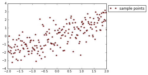
num_points = 200
X = np.linspace(-2, 2, num_points)
y = X + np.random.normal(0, 1, num_points)
plt.plot(X, y, 'r*', label='sample points')
plt.legend(loc="upper left", bbox_to_anchor=(1,1))
<matplotlib.legend.Legend at 0x10d840790>
ones = np.ones(num_points)
X_matrix = np.matrix(np.column_stack((X, ones)))
y_matrix = np.transpose(np.matrix(y))
print X_matrix.shape, y_matrix.shape
(200, 2) (200, 1)
XtX = X_matrix.transpose().dot(X_matrix)
Xty = X_matrix.transpose().dot(y_matrix)
solution = np.linalg.inv(XtX).dot(Xty).tolist()
w, b = solution
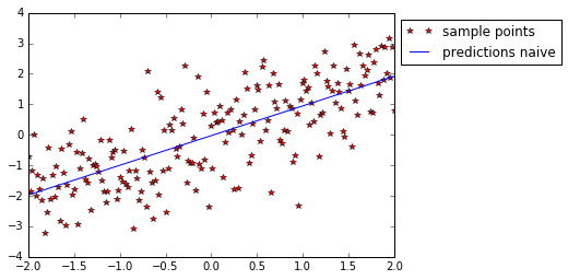
y_pred = w[0]*X + b[0]
plt.plot(X, y, 'r*', label='sample points')
plt.plot(X, y_pred, 'b', label='predictions naive')
plt.legend(loc="upper left", bbox_to_anchor=(1,1))
<matplotlib.legend.Legend at 0x10ecc46d0>
Now, tensorflow way
X_tensor = tf.constant(X_matrix)
y_tensor = tf.constant(y_matrix)
XtX_tensor = tf.matmul(tf.transpose(X_tensor), X_tensor)
Xty_tensor = tf.matmul(tf.transpose(X_tensor), y_tensor)
solution_tf = tf.matmul(tf.matrix_inverse(XtX_tensor), Xty_tensor)
sess = tf.Session()
soln_tf = sess.run(solution_tf).tolist()
w_tf, b_tf = soln_tf
y_pred_tf = w_tf[0]*X + b_tf[0]
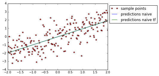
plt.plot(X, y, 'r*', label='sample points')
plt.plot(X, y_pred, 'b', label='predictions naive')
plt.plot(X, y_pred_tf, 'g', label='predictions naive tf')

plt.legend(loc="upper left", bbox_to_anchor=(1,1))
<matplotlib.legend.Legend at 0x10ede6710>